The Social Relief of Distress - How Has Poverty Changed Between 2019 and the Second Quarter of 2021?

Introduction

This brief presents a method for estimating poverty quarter by quarter and for assessing the impact of the Social Relief of Distress grant, including the supplementation of the caregiver/child support grant.

At the end of the previous brief in this series, it was noted that the NIDS-CRAM survey put the percentage of adults living in households with incomes below the food poverty line at 39.5% in January 2021 compared with the General Household Survey estimate of 32.8% in 2019. This compares these findings with the poverty estimates produced by the quarterly updating method.

Method

A simulation model produces the estimates. The model uses three data sets: the most recent General Household Survey (currently the 2019 GHS), the most recent Labour Market Dynamics Survey (currently the 2019 LMDS) and the Quarterly Labour Force Survey for the quarters in question. The Appendix sets out the technical details.

Findings

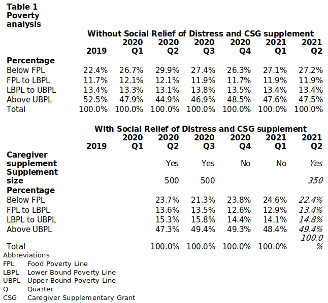
Table 1 sets out the distribution of the population according to the income of the households to which they belong.

Interpretation

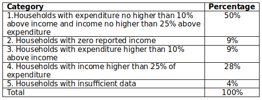
1. The accuracy of earnings data. The NIDS-CRAM data indicate that 39.5% of the adult population lived in households under the food poverty line in January 2021. This compares with 32.8% as measured by the GHS in 2019, without adjustment of zero reported incomes. The more careful analysis in this brief revises the GHS measure to 22.4% in 2019. Even so, there are grounds for suspecting some reports of very low incomes. Ideally, these should be checked against household consumption levels. Table 2 presents a check using data from the 2019 GHS.

Table 2
Distribution of households by relationship between household income and household expenditure, GHS 2019

Households in category 1 pose no problem for the analysis in this brief, since income and expenditure are broadly consistent. Neither do those in category 2 and 5, since employed people with zero reported income are assigned an imputed income. The large number of households in category 4 indicate that household expenditure was often under-reported in GHS 2019, but this has no bearing on the analysis here. It is income reporting in the households in category 3 that suggests that, even in the analysis here, some households have higher incomes than reported, the median household income in this category being R 1 275 per month, implying that most of the bottom 50% have reported per capita incomes in the poverty range. It follow that the poverty estimates presented here are a little on the high side.

2. It appears that the increase in poverty from the 2019 level started before the first COVID lockdown, with 2020 Q1 levels being substantially higher. Of course, the first lockdown made things worse again, with nearly 30% of households below the FPL, before receipt of the SRD grant, including the caregiver supplement. The SRD grant reduced the percentage under the FPL by about 6% in the second and third quarters of 2020, with a smaller reduction of about 2.5% in the percentage below the UBPL, stabilizing at close to the 2020 Q1 level in 2021

3. The pattern of SRD relief has been erratic. The R 350 grant lasted from May 2021 to April 2022, but the R 500 grant lasted only until October 2020. Moreover, the extensions to the duration of the R 350 grant beyond October 2020 were granted three months at a time. From May to July 2021, there were no grants. From August 2021 to March 2022, the R 350 grant was reintroduced, with caregivers eligible to apply. The on-again off-again nature of the relief must have affected decisions about whether it was worth applying for the grant. The more permanent the scheme is perceived to be, the higher will be the application rate, other things equal and it was reported in the first brief of this series that the take up rate is higher since August 2021 than before April 2021. As the fifth brief in this series indicated, it has a long way further up to go.

4. The termination of the caregiver supplementary grants in October 2020 meant that the impact of relief on poverty was considerably lower in 2020 Q4 and 2021 Q1 than in 2020 Q2 and 2020 Q3. There was no relief in May 2020, so the post-relief poverty levels reported for 2021 Q2 are hypothetical levels, assuming the reintroduced relief scheme in August 2021 had been in operation in that quarter.

5. The trend in poverty from quarter to quarter will depend on (a) how far the growth of earnings and social grants exceed or fall behind the increase in poverty lines and (b) how employment grows and contracts. By 2021 Q1 and Q2, the pre-relief poverty levels stabilized at a level little worse than in 2020 Q1, with earnings increase roughly balancing off unemployment increases.

6. On the whole, the relief programme has stabilized the percentage of the population under FPL at little worse than the 2019 level. The percentage under UBPL has increased more substantially, stabilizing at close to the 2020 Q1 level.

7. If there will be an average of nine million beneficiaries a month between August 2021 and March 2022, the total cost of payments will be R28.3 billion, slightly more than is to be appropriated by Parliament for the purpose. A recent document from the National Treasury^[1] puts the annual cost of continuing the scheme at R 70.9 billion rand, implying monthly expenditure of R 5.9 billion, substantially above the R 3.1 billion projected for the remainder of the 2021/22 financial year. Presumably the higher estimate is based on a 100% take up rate, or close to it. Assuming the take up rate rises to the point where R 4.5 million (the average of the two estimates) would be needed, implying an annual addition to the social grants budget of R 54 billion. This would be a substantial stretch, but would imply much less additional expenditure than a basic income grant, whose cost the Treasury projects at a wholly unaffordable R 194 million with a BIG set to the FPL.

Charles Simkins
Head of Research
charles@hsf.org.za

Appendix

1. The model is encoded in Stata Version 10.

2. As a simulation, the model extracts structure from the underlying data, and then makes certain allocations to households and individuals using random numbers within the structure.

3. The data used in the model are derived from the household and employment structure of the General Household Survey, as updated by information from the Labour Market Dynamics Survey, the Quarterly Labour Force Survey, Quarterly Employment Statistics, the National Income Dynamics Study’s Coronavirus Rapid Mobile Survey, United Nations Population Prospects 2019, social grant statistics from the South African Social Security Agency and National Treasury Budget Reviews.

4. Population and household structure. The GHS10 data set is updated to the first quarter of 2021, by adjusting for population size. The population estimated by GHS19 was 58,429,000. The United Nations World Population Prospects interpolated for the first quarter of 2021 is 59,766,000, for instance, so the adjustment factor is 1.0229. The adjustment is effected by multiplying the personal and household weights by this factor. The household structure of the population is assumed to be constant over the period between 2019 and the quarter in question.

5. Employment structure. The model classifies employees by broad occupational category. All three data sets contain information on the classification of employees across occupational categories. People owning businesses are also identified. Cross-cutting the occupational categories are gender, age, educational category, the formal/informal sector division, and geographical type.

6. The educational category uses a three way classification:

1. Up to an including Grade 9 or equivalent.
2. Grades 10, 11 and 12, or equivalent.
3. Post Grade 12 qualification.

7. The labour market status category uses a four way classification:

1. Employee, formal sector.
2 Employee, informal sector.
3. Own business, formal sector.
4. Own business, informal sector.

8. The number of employees in each occupational category will vary between the GHS as updated and the QLFS for each quarter. In some categories the QLFS number will be lower than the GHS number; in others it will be higher. Using random numbers, the model either removes the appropriate number from the ranks of the employed or adds to them from the ranks of the unemployed according to the official definition.

9. Employment updates. The number of employees in each occupational category will vary between the GHS as updated and the QLFS for each quarter. In some categories the QLFS number will be lower than the GHS number; in others it will be higher. Using random numbers, the model either removes the appropriate number by occupational category from the ranks of the employed or adds to them from the ranks of the unemployed according to the official definition.

10. Household Income components. Household incomes are made up of four components: earnings from employment and business activities, social grants, private pensions and remittances. Dividends, interest and rents are not included. This would matter if inequality were the central concern, but these components may be ignored when it comes to the analysis of poverty, since most property income accrues to persons and households which are not poor.

11. Imputation of earnings. There are many missing values for earnings in the LMDS. Were these to be accepted as zeros, there would be a substantial underestimation of household incomes, so values have to be imputed. The variables controlling the imputation are:

• Gender
• Educational category
• Labour market status
• Geotype, using a two way classification:

1. Urban
2. Traditional and farms.

Imputation is also necessary for added employment in occupational categories in which it occurs. Imputation is based on the distribution of known earnings across salary categories in the LMDS by each combination of controlling variables.

12. Income component updates. Income components are updated using indices as follows:
    Earnings. Average wages reported by the Quarterly Employment Survey
    Social grants. Average grant size, calculated from grant levels per category and the distribution of grants across categories as reported by SASSA.
    Private pensions. Average wages, except when the nominal level is below the initial level derived from the GHS, when the index is set at 100.
    Remittances. Average wages reported by the Quarterly Employment Survey.

13. Poverty lines. The three Statistics SA poverty lines are used. These poverty lines are calculated for April each year. Quarterly poverty lines are interpolated and used in order to avoid sudden jumps in measured poverty in the second quarter each year.

14. Incorporation of social relief of distress grants and caregiver supplementary grants. These are not included in the GHS19 data base, so they are added in quarters where they were payable in the middle month of the quarter. The allocation of the SRD grants was based on information in Wave 4 (January 2021) of the NIDS-CRAM survey. From this survey, a model was estimated, using age group, gender, whether employed or not, and monthly household income categories. This model produced an estimate of the probability of each person between the age of 18 and 59 receiving an SRD grant. One caregiver grant was allocated to each household in which there were one or more eligible children in the GHS as updated. For each quarter in which the SRD grant was paid, the distribution of people across the four categories divided by the poverty lines was calculated without and with the SRD and caregiver supplementary grants so that their effect can be assessed.

Annexure – Model details

Format

The model has been developed in Stata 10. It can be updated every quarter, with a few adjustments.

Data

The model is constructed from three data sets:

1. The General Household Survey 2019
2. Labour Market Dynamics 2019
3. The Quarterly Labour Force Survey 2021 Q1

It also requires a population size estimate and an update of the wage level.

Assumptions

1. The model is updated using a factor designed to bring the population up to a level computed from the United Nations World Population Prospects (most recent version is 2019) for the quarter under consideration. This means that the population structure, including household sizes, derived from the General Household Survey is assumed constant. The numbers of households and people are simply scaled up. This is an adequate approximation in the short run, but it becomes less so as time goes on. For this reason, the GHS used should not be more than two years older than the quarter under consideration.
2. The model is also updated to bring the average earnings per employee up to the level in the quarter under consideration. Three magnitudes can be considered for this purpose:

• Average earnings as reported in the Quarterly Employment Survey
• Compensation of employees as reported in the quarterly national accounts divided by the number of employed people in the Quarterly Labour Force Survey or the Quarterly Employment Survey
• Household consumption expenditure (largely financed from earnings) as reported in the quarterly national accounts divided by the number of employed people in the Quarterly Labour Force Survey or the Quarterly Employment Survey. This is the least satisfactory measure as it is influenced by consumer confidence as well as earnings.

In general, these three measures will give different estimates of changes in average earnings and the adjustment has to be based on a judgment. The earnings structure is assumed constant and all earnings are adjusted up by a constant factor. This is an adequate approximation in the short run, but it becomes less so as time goes on. For this reason, the LDS used should not be more than two years older than the quarter under consideration.

3. Like all simulation models, the model uses random numbers. For example, if employment drops by 10%, the position would be the same as in the Roman practice of decimation, the punishment for a legion which had disgraced itself in battle. The soldiers were lined up on the edge of a cliff and every tenth one was pushed over to his death. It would have had the same effect if the numbers one to a hundred had been deposited in a bucket, from which a soldier would draw, and be pushed over if his number was ten or less. If employment rises, additional worker is drawn from the ranks of the officially unemployed. The use of random numbers can obscure correlations between variables.